Check out the video below for a quick explanation of the Excel Vlookup function. Or, if you’d rather read, the video is summarized further down the page.
Video summary
The Excel function Vlookup’s name comes from Vertical LOOKUP. We look up the score of a person in a table.
The arguments
The first argument is the value that we’re looking up. Ann in this case. Click on the cell containing Ann. The second argument is the complete table that we want to look into, except for the headers.
The third argument is the column index number, the index of the column of the value that we want to return. This means the how many-th column the value is in that we want to show as a result. We want to show the score, which is in the second column, so we use 2.
The final argument is the (optional) Range lookup argument. Using false will make Excel look for the exact value, using TRUE will make it look for an approximate match. You almost always want to use FALSE here. Check out the Questions section below for when you should use TRUE.
Errors
If the lookup value does not exist, Excel will show a #N/A (Not Available) error.
More on Vlookup
Syntax
=VLOOKUP (Lookup value,Table array, Column index number, [Range lookup])
Argument | | Argument description |
|---|---|---|
1 | Lookup value | Value to search for (must be in first column of the table). |
2 | Table array | The table to look in. |
3 | Column index number | How many columns away the returned value is from the lookup value. |
4 | Range lookup | Approximate (True) or precise (False). |
Another example
Suppose you want to look up the scores of two students. You have a table containing the scores of all the students of the course on another worksheet. But you don’t want to look them up yourself, you want Excel to do it for you.
Use the VLOOKUP function to search for the scores of the two students.
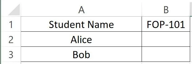


The two students Alice and Bob. We want to know their FOP-101 score.
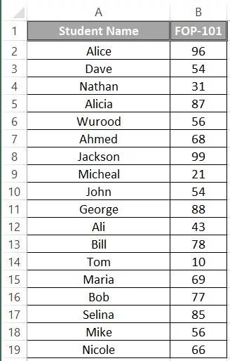


The complete table of students and their scores.
Answer
Use =VLOOKUP(A2, ScoreSheet!A1:B19, 2, FALSE) in cell B2 to look up the score of Alice.
Explanation
Questions about Vlookup
Why is using FALSE for the Range lookup variable a good rule of thumb?
Because almost always, we want to look for exactly the thing we have as our reference. Looking for almost the value can lead to unexpected results. Read the answer below to see when you would want to use TRUE for this.
When SHOULD you use TRUE for the Range lookup variable for Excel’s VLOOKUP?
When the table you are using VLOOKUP on has values that correspond to ranges of numbers. For example: 0 – 10 Low,10 – 20 Medium,20 – 30 High.If you have value 15, the result should be Medium. In this scenario, a vlookup with value 15 will return Medium if you set Range lookup to TRUE but not if it’s set to FALSE.
What happens when the lookup value does not exist in the table?
If the lookup value doesn’t exist, Excel will show a #N/A error in the cell where the Vlookup function is used. You can ‘catch’ this error using for example the IFERROR function.
Drawbacks and how to overcome them
The Vlookup function has some drawbacks:
- The Vlookup function will only look for the lookup value in the leftmost column of the lookup table. But what if you want to look up a value in the second column? You will have to reposition the table array argument to have its leftmost column one position further.
- The Vlookup function will only look to the right of the lookup value in the table. You will have to change the table layout if you want to look to the left of that column.
That’s it
That’s all for Vlookup. Did we help you understand this function? Do you have other techniques to look up values in Excel? Let us know in the comments.
Also, if you enjoy this type of content, you might want to look at some more Excel learning material.


1 thought on “VLOOKUP explained in 2 minutes”