Beginners Excel tips and tricks

You’ve worked with Excel a few times. You’ve seen others use it to great effect. And now, it is your time to start on your path to becoming the Excel guru of the office.

Welcome to the beginners tips and tricks for Excel.

Let’s get right to it.

1. Drag and drop to move

A lot of people use cut and paste to move cells in an Excel worksheet. If they’re feeling adventurous they may even use the keyboard shortcuts to do so.

What these people don’t know is that you can also drag and drop to move cells. To do this, select some cells, click on the edge of the selection and drag to a new position.

Drag and drop cell moving.

2. Counting, summing and averaging without formulas

A quick way to count, sum or average without writing a formula is by selecting the cells you are interested in and looking at the status bar. The status bar is the bar at the bottom of the Excel window.

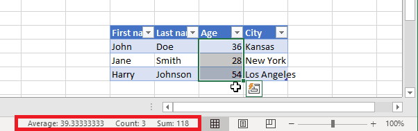
The status bar shows the average, count and sum of the currently selected cells. You click on this image to zoom in.

You can even adjust the values that are shown by right clicking on the status bar. In the menu that appears, you can choose any configuration of the defaults (average, count and sum) and numerical count, minimum and maximum as well.

3. Fixing rows

This one is most useful when you’re working with large tables. By fixing the headers of the table, you’ll be able to scroll through the table while still seeing what every column represents.

Here’s how you do it:

This may seem counter-intuitive, but select the cell(s) positioned one cell below the row you want to fix.
Go to the View tab on the Ribbon and click on Freeze Panes.
Click on Freeze Panes in the dropdown that shows.

Freezing the headers of the table/cell range.

Important note about Freeze Panes: this isn’t the whole story of Freeze Panes. All cells that are above or to the left of the cell that is selected when you click Freeze Panes will be fixed.

In the video above, there are no cells to the left of the selection. However, if you would select cell B1 before clicking Freeze Panes, you will freeze the complete A column. That’s because it is to the left of B1.

So you can use this same trick to fix columns as well.

4. Inserting multiple rows & columns at once

If you didn’t know, you can insert rows and columns by right clicking on the row or column header (the 1,2,3 or A,B,C part) and selecting Insert.

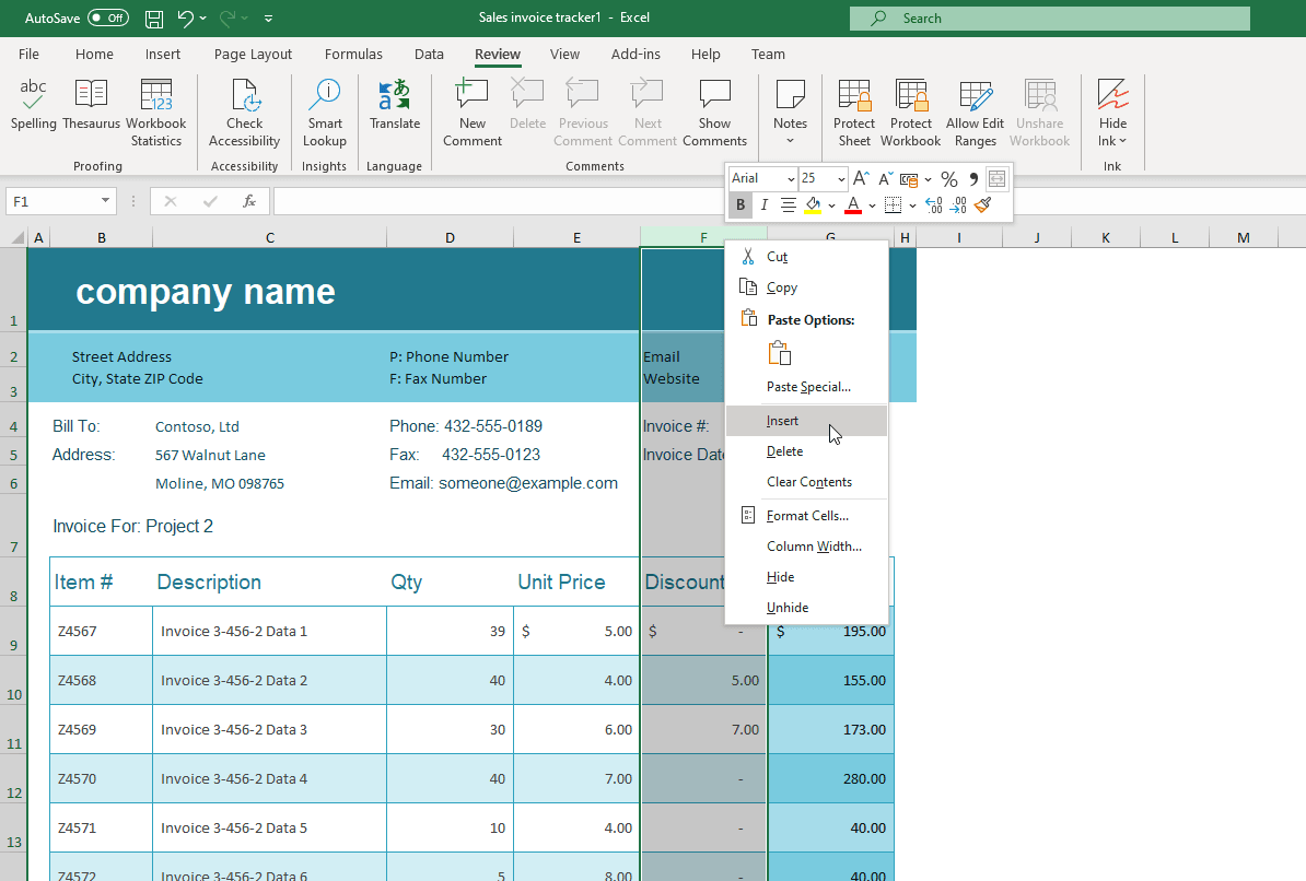
Inserting a new column. You click on this image to zoom in.

For rows, this will create a row above the row you right clicked on. For columns, it will create a new column to the left of the column you right clicked.

All other cells will be moved down (when inserting a row) or to the right (when inserting a column).

Now, for inserting multiple rows and columns at once.

All you have to do is select more rows before right clicking and Inserting. Or more columns. So if you want to insert three rows, select the three rows below the position where you want to insert the new rows. Then, as before, right click and select Insert.

5. Combining cell contents

Without knowing too much about functions and formulas, you can still easily combine the contents of two cells.

Use the formula: =A1&" "&B1 to combine cells A1 and B1 with a space in between.

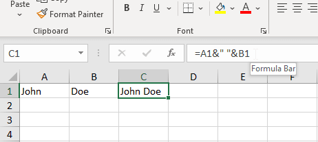
Using the formula =A1&” “&B1 to combine the contents of cell A1 and B1.

As you might expect, you can change A1 and B1 for any other cells and it will still work.

6. Transposing

If you’re unsure of what transposing means, it is basically switching rows and columns around. A row becomes a column and a column becomes a row. You’ll understand when you see the video in a second.

So when do you use transposing? It can be useful when your table is very wide and you want it to be long instead for easier scrolling. Or when it simply improves readability. Or if you want to use VLOOKUP instead of HLOOKUP.

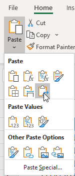
To transpose a table or cell range in Excel:

Select the cells that you want to transpose
Copy them using Ctrl + C (Windows) or ⌘Command + C (Mac) or alternatively by clicking on Copy on the Home tab of the Ribbon. Make sure you don’t cut instead of copy, that won’t work.
Select a cell with a large empty space to its right and down (the transposed table has to fit here).
Click on the arrow below the Paste button on the Home tab of the Ribbon.
Click on Transpose (the clipboard with arrows to the right and down) in the dropdown that opens.

The Transpose option in the Paste dropdown.

Transposing a table by selecting it, copying and pasting it transposed.

Where are the other tips?

We’re still working on this page. Therefore, only the tips and tricks until this point are available.

Sorry for the inconvenience, you can check out the [thrive_2step id=’2112′]Excel Beginner Cheat Sheet[/thrive_2step], which contains more beginner tips.

Those have been the beginner tips and tricks

By reading this far, you’ve seen many useful Excel tips that will give you a nice start to building your Excel knowledge. We hope you’ve noticed and appreciated how quick and to-the-point the explanations were.

Here’s a little secret: many of these tips have been taken directly from the Excel Foundation Course. If you like the way they were explained you’d enjoy the full course.

If you don’t get the full course, that’s fine as well! If you enjoyed the tips though, please share this page with people that could benefit from it.

What’s next?

You can try your hand at the Intermediate Lesson.

Happy Excelling!